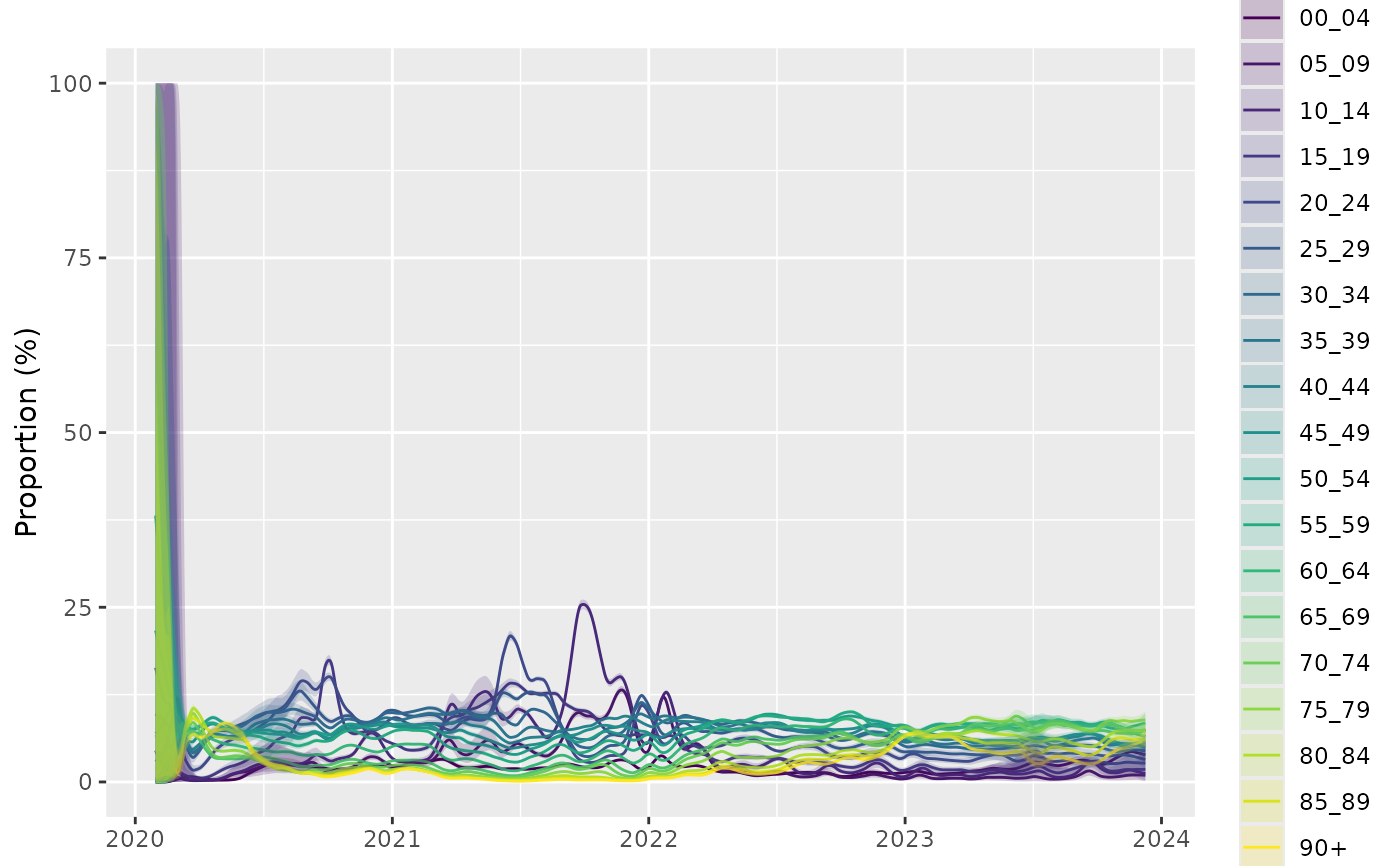
Plot a proportions timeseries

Usage

plot_proportion(
  modelled = i_proportion_model,
  raw = i_proportion_data,
  ...,
  mapping = if (interfacer::is_col_present(modelled, class)) ggplot2::aes(colour = class)
    else ggplot2::aes(),
  events = i_events
)

Arguments

modelled

Proportion model estimates

A dataframe containing the following columns:

time (as.time_period + group_unique) - A (usually complete) set of singular observations per unit time as a `time_period`
proportion.fit (double) - an estimate of the proportion on a logit scale
proportion.se.fit (double) - the standard error of proportion estimate on a logit scale
proportion.0.025 (proportion) - lower confidence limit of proportion (true scale)
proportion.0.5 (proportion) - median estimate of proportion (true scale)
proportion.0.975 (proportion) - upper confidence limit of proportion (true scale)

No mandatory groupings.

No default value.

raw

Raw count data

A dataframe containing the following columns:

denom (positive_integer) - Total test counts associated with the specified timeframe
count (positive_integer) - Positive case counts associated with the specified timeframe
time (as.time_period + group_unique) - A (usually complete) set of singular observations per unit time as a `time_period`

No mandatory groupings.

No default value.

...

Arguments passed on to geom_events, proportion_locfit_model

window: a number of data points defining the bandwidth of the estimate, smaller values result in less smoothing, large value in more. The default value of 14 is calibrated for data provided on a daily frequency, with weekly data a lower value may be preferred. - (defaults to 14)
deg: polynomial degree (min 1) - higher degree results in less smoothing, lower values result in more smoothing. A degree of 1 is fitting a linear model piece wise. - (defaults to 1)
frequency: the density of the output estimates as a time period such as 7 days or 2 weeks. - (defaults to "1 day")

mapping

a ggplot2::aes mapping. Most importantly setting the colour to something if there are multiple incidence timeseries in the plot

events

Significant events or time spans

A dataframe containing the following columns:

label (character) - the event label
start (date) - the start date, or the date of the event
end (date) - the end date or NA if a single event

No mandatory groupings.

A default value is defined.

Value

a ggplot object

Examples

tmp = growthrates::england_covid %>%
  growthrates::proportion_locfit_model(window=21) %>%
  dplyr::glimpse()
#> Rows: 26,790
#> Columns: 12
#> Groups: class [19]
#> $ class                  <fct> 00_04, 00_04, 00_04, 00_04, 00_04, 00_04, 00_04…
#> $ time                   <time_prd> 0, 1, 2, 3, 4, 5, 6, 7, 8, 9, 10, 11, 12, …
#> $ proportion.fit         <dbl> -13.433629, -13.178345, -12.898497, -12.600007,…
#> $ proportion.se.fit      <dbl> 51.598289, 49.954079, 48.024633, 45.878749, 43.…
#> $ proportion.0.025       <dbl> 1.759164e-50, 5.698079e-49, 3.308357e-47, 2.991…
#> $ proportion.0.5         <dbl> 1.465037e-06, 1.891110e-06, 2.501801e-06, 3.371…
#> $ proportion.0.975       <dbl> 1.0000000, 1.0000000, 1.0000000, 1.0000000, 1.0…
#> $ relative.growth.fit    <dbl> 0.24102860, 0.24048966, 0.23901181, 0.23680352,…
#> $ relative.growth.se.fit <dbl> 1.2309119, 1.2257057, 1.2114298, 1.1900979, 1.1…
#> $ relative.growth.0.025  <dbl> -2.1715143, -2.1618494, -2.1353470, -2.0957455,…
#> $ relative.growth.0.5    <dbl> 0.24102860, 0.24048966, 0.23901181, 0.23680352,…
#> $ relative.growth.0.975  <dbl> 2.6535715, 2.6428288, 2.6133706, 2.5693525, 2.5…

plot_proportion(tmp)+
  ggplot2::scale_fill_viridis_d(aesthetics = c("fill","colour"))